Context

• The most common techniques for deep learning model compression are pruning and quantization.

• Model compression can significantly reduce model size and latency without significantly impacting top-line metrics, e.g., global accuracy.

• The paper investigates if model compression may systematically affect performance on specific datapoints or classes.

Takeaways

• Some datapoints and classes are indeed more affected by compression.

• A larger portion of the performance degradation concentrates on:
  • Challenging examples (either for humans or uncompressed models);
  • Classes with fewer examples.

• Compressed models are less robust to domain shift than their uncompressed counterparts. They ran experiments with image corruption or adversarial examples.

• Quantization is less harmful than pruning.

My remarks

• I don’t really understand the value of their discussion on corruption and adversarial examples. They compared the compressed model with the uncompressed one and observed that the latter is better. But this was, of course, expected. After all, the compressed model has a smaller capacity.

• A more interesting (and maybe fairer) comparison is to compare a pruned model with a model of the same size trained without pruning. My bet is that the pruned model would be more robust.

• The way the paper was written gives the impression that compression is bad for domain shift robustness. But it may be just the opposite. For a fixed final model size, training with pruning may result in increased robustness compared to training with the fixed model size from the beginning.

Takeaways

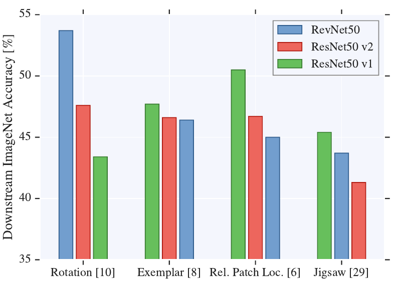
• The paper presents a large empirical study comparing different self-supervised techniques and neural architectures (all CNNs; this is a 2019 paper).

• Increasing the number of filters consistently improves performance. This is similar in the fully-suppervised scenario. But in self-supervising the effect is even more pronounced. Accuracy improvements were observed even in the low-data regime.

• Overall, the performance on the pretext task is not predictive of the performace on the downstream task.

• For ResNets, the downstream accuracy is higher when using the representations obtained from the last layer (the one before the “logits layer”, which, in turn, is task-specific).

• On the downstream task, an MLP performed just marginally better than a simple linear classifier (logistic regression).

• Training the logistic regression to convergence can take a lot of epochs. They saw improvements even after 500 epochs.

Takeaways

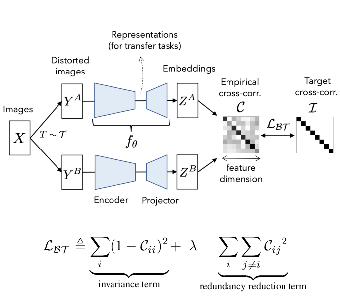
• The paper proposes a new loss function for self-supervised learning.

• It is based on the cross-correlation matrix (CCM) of the outputs of two identical networks fed with two distorted versions of the same image. See the image above.

• The loss value is minimal when the CCM is equal to the identity.

• Having the CCM’s main diagonal elements equal one means that the network outputs are invariant to each other. Therefore invariant to the distortions.

• Having the off-diagonal elements equal zero means that the output dimensions are uncorrelated. Therefore the information redundancy is zero. This constraint avoids the training collapse (i.e., when the network ignores the inputs and always outputs a constant prediction.)

• Barlow Twins are very simple and easy to implement. Still, it performs competitively or outperforms other state-of-art methods.

Takeaways

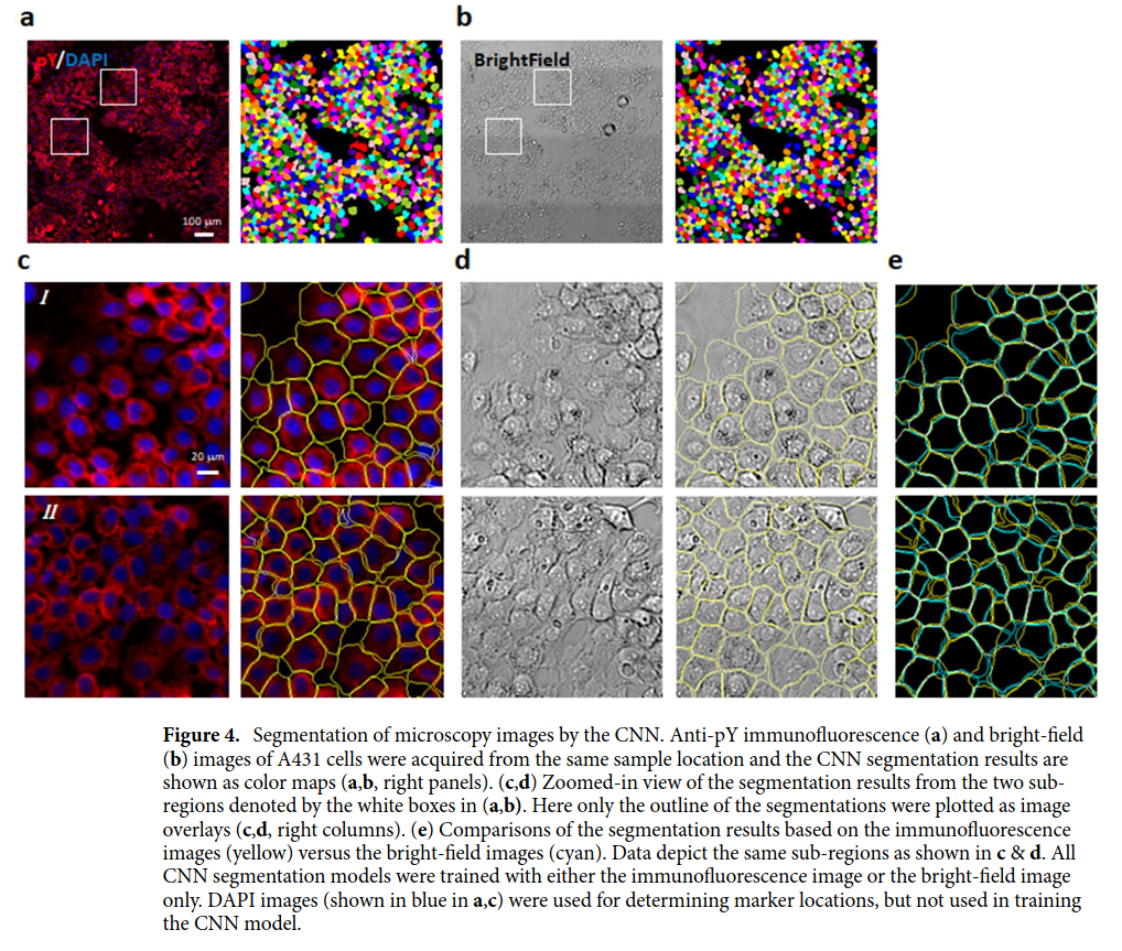
• The paper proposes a loss function to train neural networks (e.g. U-net) for single-cell image segmentation without labeled data (i.e. unsupervised learning).

• The input images (see figure above) are from 2D cell cultures (i.e. cell monolayers). The cells are generally packed together, but some empty spaces between them may occur.

• The method requires knowing beforehand the position of the cell’s centers and where empty spaces (i.e. the background) lie. Therefore, although the technique is said to be unsupervised, it requires some labeled data. Nevertheless, the paper uses techniques to get these labels automatically. No manual labeling is required.

• The cell’s nucleus location is used as an approximation of the cell’s center. The position of the nucleus is determined from images stained with DNA binding dye DAPI.

• The background is segmented with a traditional algorithm (graph-cut).

• During training, the full microscopy image is divided into small patches centered at each cell nucleus. The patch is just big enough to display the entirety of a single cell. The objective of the network is to segment only that single cell.

• The loss function can be expressed as the weighted sum of three costs:
  • Overlapping segmentation of different cells. This makes sense. The cells are distributed in a monolayer, so indeed there is no overlapping.
  • Cell segmentation invading the background region. Again, the background segmentation is known a priori (via graph-cut).
  • Segmenting cells with a small area. This cost is especially required to avoid the trivial solution of having no cell segmented at all.
• The paper reports an mIOU of 82.1% on their own dataset.

Context

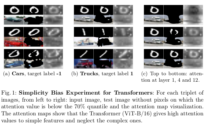
• It is often claimed that vision transformers (ViT) surpass convolutional networks (CNN) in calibration, robustness to covariate shift, and out-of-distribution (OoD) performance.

• This paper questions the methods to reach these conclusions and proposes new experiments.

• The models compared were: ConvNeXt and BiT (CNNs) vs. vanilla ViT and Swin Transformer (ViTs).

Takeaways

• ViTs and CNNs are both susceptible to simplicity bias (a.k.a. shortcut learning). See figure above.

• ViTs and CNNs perform just as well on OoD detection tasks.

• No single model exhibited the lowest Expected Calibration Error (ECE) in all covariate-shift experiments. Also, the model with the highest accuracy is not the most calibrated.

• A low ECE is not enough to assess a classifier’s reliability. It is better to complement this analysis with other techniques, such as the Prediction Rejection Ratio (PRR).

• The robustness contest between CNNs and ViTs seems to have no clear winner.

Context

• This paper was published shortly after the hype explosion around vision transformers (mainly the vanilla ViT and the Swin Transformer) as an alternative to convolutional networks.

Takeaways

• A “modernized” ResNet (named ConvNeXt) can perform equally or superiorly to ViTs.

• The ConvNeXt also performed as well as ViTs when pre-trained on large datasets, which challenges the view that ViTs are better at scaling up.

• In general, CNNs have a more straightforward design (less specilized modules) and do not use the global attention mechanism, which has a quadratic complexity dependency on the input size.

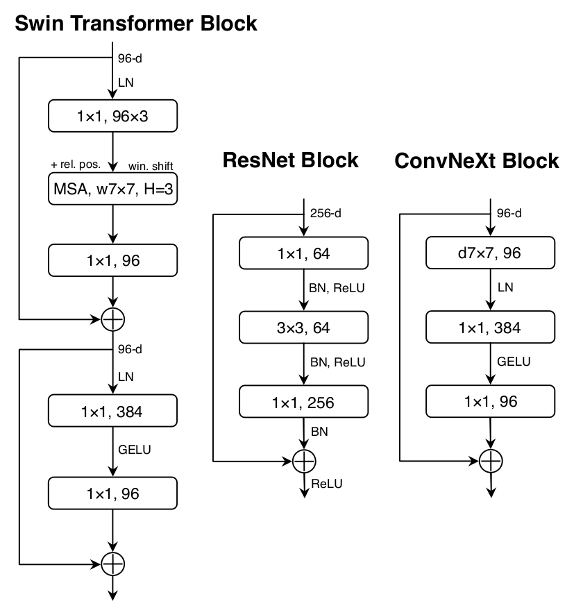
• Proposed modifications to the ResNet architecture:
  • Change the number of blocks per stage to (3, 3, 9, 3). Originally it was (3, 4, 6, 3).
  • Use a 4 x 4 convolution with stride 4 (non-overlapping convolution) as the ResNet stem cell.
  • Use grouped convolutions (a là ResNext), more specifically, depthwise convolutions, in the first layer of the block.
  • Use larger convolutions — 7 x 7 instead of 3 x 3.
  • Restructure the block as an inverted bottleneck: a layer with many filters sandwiched between two layers with fewer filters.
  • Use just one activation function per block and replace the ReLU with GELU.
  • Use layer norm instead of batch norm.
  • Insert spatial downsampling layers (2 x 2 conv with stride 2) and normalization layers between each stage.
  • The figure above (taken from the paper) shows the ConvNeXt block compared to the ResNet’s and the Swin Transformer’s.
• The training recipe was also modified:
  • 300 epochs instead of 90.
  • AdamW optimizer.
  • Learning rate linear warm-up followed by a cosine decay.
  • Data augmentation: mixup, cutmix, randaugment, and random erasing.
  • Regularization with stochastic depth and label smoothing.

Context

• It’s often said that learning methods perform better when interpolating the training data and worse when extrapolating it. This paper defies this notion.

• Definition: A model interpolates if the input lies within (or on the face) of the convex hull “wrapping” the training data. The model extrapolates if the input is outside of this convex hull.

Takeaways

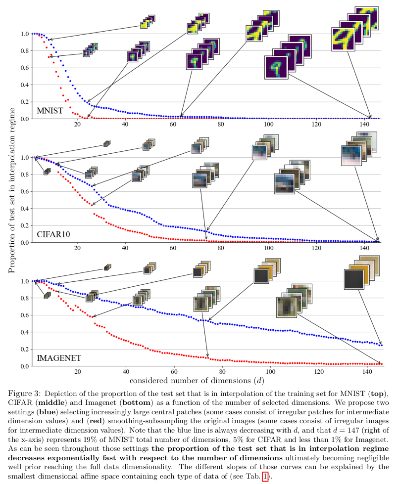
• When learning in higher dimensions, interpolation rarely occurs. The models are almost always extrapolating. They prove that with theory and experiments using synthetic and real data.

• “Higher dimensions” means more than 100. Even the smallest popular image datasets have more dimensions than that. For instance, MNIST has 784.

• To remain in the interpolation regime, the training dataset size has to scale exponentially proportional to the data’s dimensionality.

• Interpolation is unlikely to happen even in lower-dimension embedding spaces.

• Since models like deep learning handle high-dimensional data well, and these models are almost always extrapolating, it follows that considerations about inter/extrapolation are irrelevant for predicting performance.

My remarks

• The convex-hull definition of interpolation seems too strict to be useful in high-dimensional spaces. An extreme value at a single dimension (i.e. pixel) is sufficient to place a datapoint out of the convex hull.

• The convex-hull criterium gives us a hard (binary) indication of interpolation.

• A soft metric would probably be more helpful — something like the distance between the datapoint and the convex hull.

• Such a metric may better predict the per-datapoint performance.

My remarks

• Excellent paper for beginners. But more experienced researchers may also profit from this reading, given how common some of those pitfalls are.

• Some of the recommended practices are difficult to apply to deep learning because they require training and evaluating multiple models. The computational costs may be prohibitive. Nevertheless, it is vital to understand the limitations of single evaluations.

Takeaways

• Before building the model:
  • Understand the data. Make some exploratory data analysis on the training set. If the dataset is described in a paper, read it.
  • But don’t look into the test set.
  • Check if you have enough data. If not, you could generate more with data augmentation techniques and use cross-validation for a more efficient use of the existing data.
  • Talk with domain experts. It may prevent you from tackling the wrong questions or formulating your ML problem in the wrong way.
  • Review the literature. Someone else may have already solved your problem. Also, your method may have already been tried with a negative outcome.
  • Keep in mind how you want to deploy your model. Are there any time, memory, or energy constraints?
• Building the model:
  • Make sure the test data will not leak into the training process. The test dataset should be used just for the model’s final evaluation. For things like hyperparameter optimization or learning curve monitoring (e.g. for early stopping) use a validation dataset (or cross-validation).
  • Try different models. This is easy to do with libraries like scikit-learn. There is no single best ML model for all problems.
  • But don’t use inappropriate models. Models have assumptions. Check if your problem complies with these assumptions.
  • Tune the model’s hyperparameters. There are many tools out there that do this automatically (AutoML).
• Evaluating the model:
  • Evaluate the models multiple times. ML models may be unstable. Train multiple models with different random seeds and cross-validation. Evaluate all of them and report results in terms of mean and standard deviation.
  • Carefully choose the evaluation metric. For instance, don’t use accuracy with imbalanced data; other metrics, such as Cohen’s kappa coefficient (k) and Matthews Correlation Coefficient (MCC) are better suited for this situation.
  • Consider using an ensemble of models. Ensemble learning techniques, such as boosting, bagging, and stacking, are known to perform well in many situations.
• Comparing models:
  • A higher accuracy does not necessarily mean a better model. When comparing two models, one has to evaluate both models many times and use statistical tests, such as McNemar’s test, to compare their performance.
  • Use a correction factor when comparing multiple models. If you are comparing more than two models using a series of pair-wise statistical tests, you have to use a correction factor such as the Bonferroni correction to account for the multiplicity effect.
  • The results from community benchmarks may be misleading. There is no guarantee that the researchers used the test set just once. Also, small performance improvements may not be statically significant.
  • Even statistical tests may be misleading. Different tests may yield different conclusions. Also, given enough data, it is easier to make small performance differences seem statistically significant. It is beneficial to include a measure of effect size, such as Cohen’s d or the Kolmogorov-Smirnov statistics.
• Reporting the results:
  • Be honest and transparent. It is good to share your code along with a script that runs all the experiments used in your paper. Write clean and well-documented code.
  • Report performance in many forms. Use multiple datasets and performance metrics.
  • Don’t make claims not supported by the data. There are limits to what can be inferred from an experimental study. If a model performs well on a dataset it does not mean it will also do so in the real world or even on another dataset.
  • Look inside your model and try to understand how they reach their decisions. This will enrich the scientific contribution of your work. For deep learning, one could try explainable AI (XAI) techniques.

Takeaways

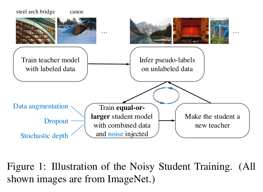
• The paper proposes a semi-supervised technique named “Noisy Student Self-learning.” It is meant to be used when large amounts of unlabeled data is available in addition to a the labeled dataset.

• It is a iterative process (see figure above). First a model is trained solely on the labeled data. Then this model takes the position of a “teacher” and is used to generate pseudo-labels for the unlabeled dataset. Next, a “student” model is trained on the union of the labeled and pseudo-labeled datasets. Most importantly, the student training should be noised (they used dropout, stochastic depth, and data augmentation). Finally, the student becomes a teacher, relabels the unlabeled dataset, and a new student is trained. They repeated this cycle three times.

• Dataset relabeling is done without noise.

• Noise while training is vital. The conditions for learning have to be harder than the conditions for generating the labels. This is what allows the student to surpass the teacher. Data noise forces the student to learn predictions invariant to augmented instances of the images. And model noise forces the student to mimic an essemble decision maker (the complete teacher) with only a fraction of its model.

• The student can be larger or as large as the teacher. There is a small benefit in using larger students, but using models of the same size works well too.

• It is better to train jointly on the labeled and pseudo-labeled dataset, than to do it first on the labeled than on the pseudo-labeled.

• The more unlabeled data the better.

Takeaways

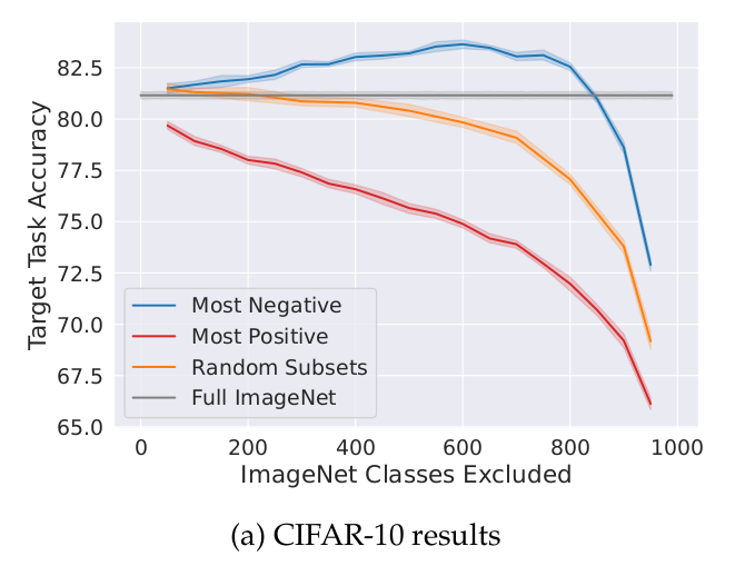
• When doing transfer learning, removing parts of the source dataset may increase the performance on the target dataset.

• To determine which parts of the source dataset to remove one can train many models on different subsets of the source dataset. In each subset, some classes are removed at random. After evaluating each model on the target dataset, one can estimate the benefit of each source class by calculating the mean accuracy of the models when the class is present minus the mean accuracy when the class is absent. (Note: In this paper, they just studied the classification problem. They also focused on removing whole classes from the source dataset, instead of individual datapoints.)

• On the ImageNet to CIFAR-10 transfer, the target accuracy improves by 2.5% when removing approximately 600 classes from the source dataset (see image above).

My remarks

• It is an interesting method, but it may be difficult to use in real applications because it requires training the model on the source dataset (which is normally large) many times. For instance, in the paper, they trained 7540 models.

Context

• It is a common practice in the machine learning community to report results from a single run (a single random seed). This many compromise the statistical validity of the presented results.

Takeaways

• The random seed has an important influence on the final accuracy of computer vision models.

• The accuracy difference between a “bad seed” and a “good seed” was around 1% on the studied benchmarks. But the gap may be even higher if more seeds were evaluated.

• Dependending on the benchmark, improvements greater than 0.5% on the current state-of-art method are generally considered relevant by the computer vision community.

• It is recommended that studies evaluate many runs with different random seeds. The accuracy should be published in terms of average, standard deviation, and minimum/maximum values.